Stravart: Making Strava Art in Python
Strava. The sport social networks, where sunday amateurs and professional athletes meet. Much like any other social networks where a mass of anons follows a few stars, but with all the data for you to know how far you are from ever becoming professional. Though with some luck and sweat, you might find yourself performing better than one of your connection on that one little segment.
In the wake of Moneyball Strava has become the perfect platform for the revenge of the data nerds over the sport bros. And if it provides all the necessary tools to build data-driven tailored programs for amateurs or athletes, we can also make Strava a bit more fun with some maths.
Perhaps one of the most well known example of such Strava fun is Strava art, where an activity’s map represents an image. If you are going to suffer running or riding, you might as well make it look nice. You can find a great collection of such activities here.
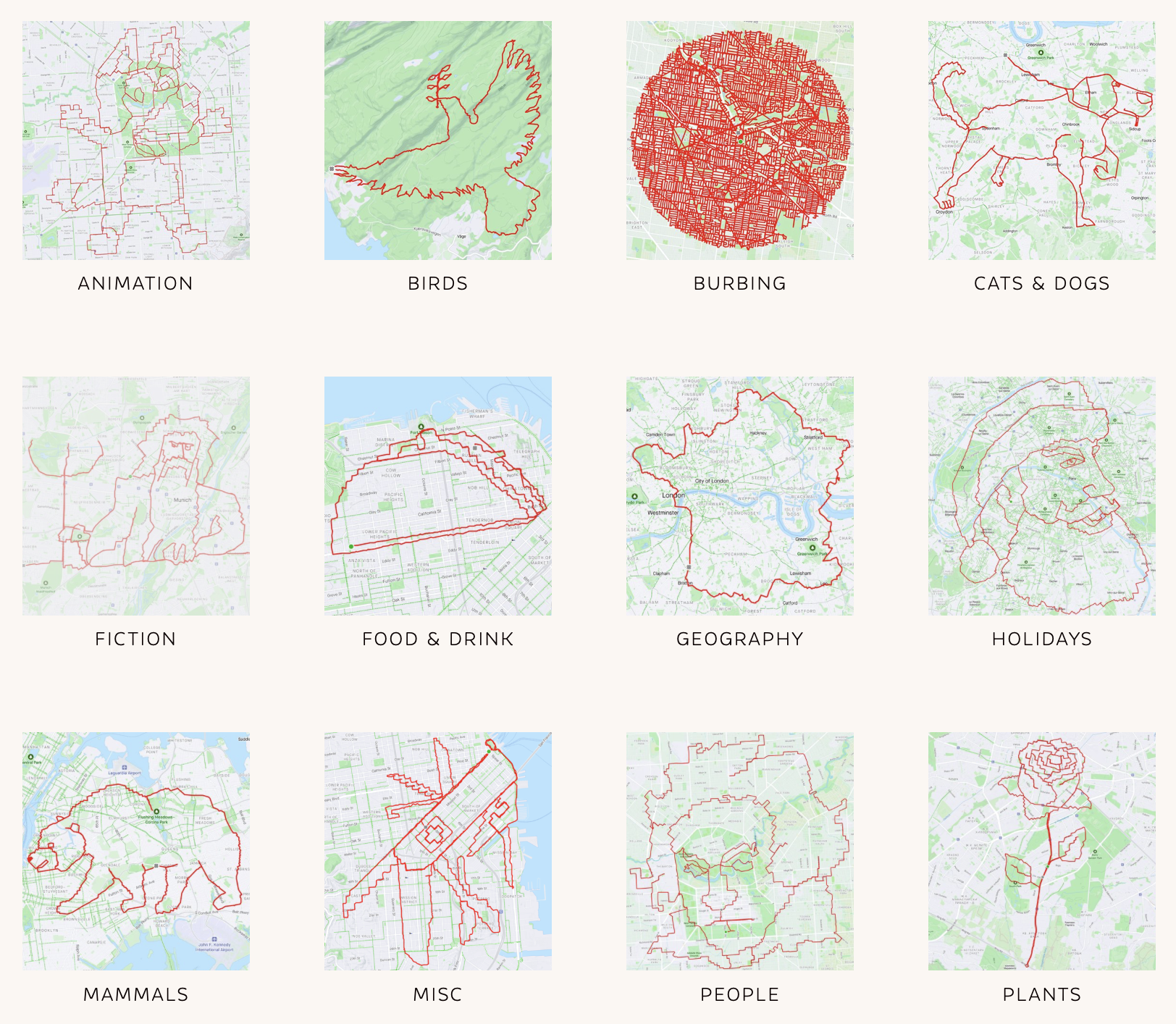
If I’ve known about this for quite a while, it’s only when I saw this thumbnail on my YouTube recommendation that I wondered how do people make those?
Much to my surprise, I couldn’t find the automated solution I was hoping for. It seems you have to reach out to gifted (and patient) artists willing to draw those manually on some maps. Perfect chance for a little holiday project!
Understanding the Problem
We have as input an image, say that of a shark, together with a location, say Paris center, we want to output a rideable path that represents that shark.
Immediatly we can decompose this into two well-separated tasks:
- Extracting a line contour from an image (that is a list of coordinates points representing the contour)
- Projecting the extracted contour onto a map into a rideable path.
A rideable path is a path that can be actually ridden (I’m a cyclist, not a runner). This means, you cannot cut through building, a river or enter a highway. Thankfully using routing services such as Google Maps or Mapbox will ensure riddeability, but there is no guarantee that the output path is close to the extracted contour as this depends quite naturally on the local topography.
Crafting a Contour Extraction Heuristic
When it comes to classical computer vision1, the most versatile tool is surely OpenCV. The standard preprocessing steps are converting to GrayScale format, applying some Gaussian blur filter, and then some canny edge detector, before finally invoking the almighty findContours.
import cv2

image_path = "/path/to/your/image.png"
image = cv2.imread(image_path)

gray = cv2.cvtColor(image, cv2.COLOR_BGR2GRAY)
blurred = cv2.GaussianBlur(gray, (9, 9), 0)
edged = cv2.Canny(blurred, 10, 100)

contours, _ = cv2.findContours(edged, cv2.RETR_TREE, cv2.CHAIN_APPROX_SIMPLE)
We immediatly see the method dependence on the choice of hyperparameter values. Unfortunately, there is no sound way to set those automatically for any images, unlike Machine Learning, we don’t have metrics at our disposal here to guide us.
ThefindContours methods detects all possible contours in the image which might not be what we are after. Imagine there are some little fishes by the shark. Or that the shark is detected as multiple contours like this
This is why we set up the following heuristic. After all contours are detected, we start by merging all contours that share points, we then merge the largest contour with all other contours whose distance is below a given threshold (5% of the image’s width by default).
The last step is to control the size of the contour. The more points the contour has, the more complex (or at least expensive) the projection onto a rideable path will be. To resample the contour, we can use the beautiful Ramer-Douglas-Peucker algorithm2… although here again there is a parameter, the distance dimension epsilon, to be set, whose natural unit is the contour perimeter. In my very small scaled experiments, to be sure to keep all distinguishing feature of the contour, I’ve found eps=0.001 to perform reasonably well.
epsilon = eps * cv2.arcLength(merged_contour, True)
simplified_contour = cv2.approxPolyDP(merged_contour, epsilon, True)
When we think we done, we think again. This pipeline works well but under the implicit assumption that the input image is already representing a contour. If we are instead dealing with natural images, just like those cats below, we can leverage the best and latest deep learning models to perform panoptic segmentation like Mask2Former:
 |
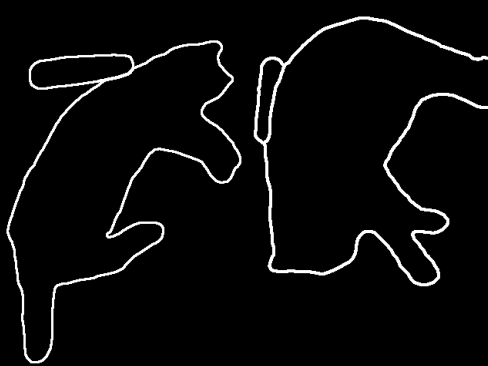 |
Once we land on the contours of the right-hand side image, we can go back to the first described pipeline.
Searching for the Best Route
To project the newly found contour - really just a list of coordinates- onto a map, we need two elements: one point of the map to center the projection, and a maximum distance to bound the projection. This means that the contour is included in the sphere center on the point with radius the maximum distance. As we explained above, this doesn’t give a rideable path.
The first thing to do is to get biking directions between every consecutive pair of points in the contour. This can be achieved with any geolocation and directions providers (Google Map, MapBox, Open Street Maps) and yield a rideable path. However we might end up with a path that looks nothing like our image contour.
We can explore other nearby rideable solutions by moving around the map center and relaxing the maximum distance. We can also apply some geometrical operation on the contour like small rotations or distortions. If this provides us with a set of rideable solutions, in order to choose one, we need to define what the best rideable solution means. We need a metric to quantify the discrepancy between the original first contour and the contour of the rideable solution.
There are many existings metrics to compare two paths such as Hausdorff, Fréchet or Wasserstein’s distance. However they don’t capture the semantic similarity we are looking for as we only care for the rideable solution’s contour to suggest the original image shape. We set up on the following similarity measure.
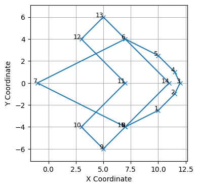
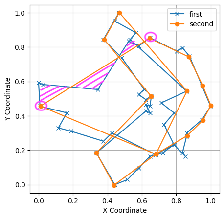
Going through the original contour, for each pair of successive points, we compute the area of the polygone defined by this pair together with all the intermediate points suggested by the routing algorithm to travel from the first to the second point. More visually, for the pair of points circled in pink in the below contour, this area is polygone is represented by the pink shaded zone.
 |
 |
We now have all the pieces to search for the best rideable path representing our image contour. The parameter space to search over is made of:
- A grid of points over a desired location,
- An interval
[min_angle, max_angle]for the rotation angle, - An interval
[radius_min, radius_max]for the projection radius.
We can then use our favorite hyperparameter optimization algorithm, whether simple random search or fancy bayesian methods. I’ve chosen Optuna for their nice intuitive API which by default uses TPE (Tree-Structured Parzen Estimators).
Introducing Stravart
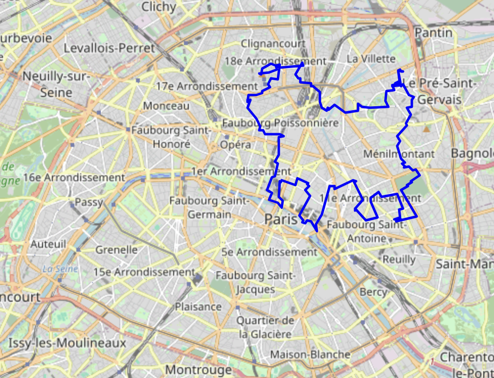
All the above experiments made it into a toy Python package I’ve developed3 called stravart. Every step of this post is detailed in a separate notebooks (whether contour extraction or hyperparameter optimization). There is even a small streamlit webapp that displayed the optimization process on a map. I initially wanted to make this available as a service, deployed on a website but I haven’t managed to get to it yet…
 |
 |
LLM Bonus
Of course, I tried my luck with the latest LLMs and directly prompt them to do the entire task: output a list of coordinates centered on Paris that represents a shark.
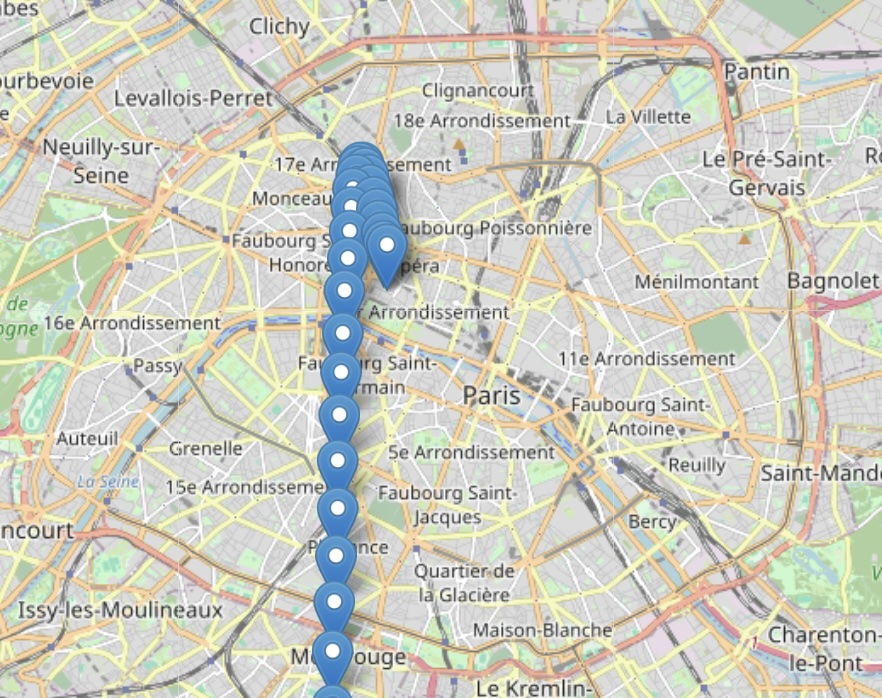
Both mixtral-8x7b and gpt-4 kindly obeyed my command and gave me list of coordinates. While it was correctly centered on Paris, it didn’t quite looked like a shark:
So maybe AGI is not just around the corner after all…