In Search of Causal Metrics
When leaving the realm of traditional Machine Mearning to join the shore of Causal Inference, it’s not the fancy deep learning algorithms that we ultimately miss the most, it’s the metrics. Without metrics, without statistical learning theory, no performance guarantee.
As a direct consequence of the fundamental problem of causal inference, it is impossible to evaluate what we partially observe. The very notion of ground truth disappears. If a policy suggests a treatment different than the one a unit actually received, how can we tell which treatment allocation is the best one?
Causal Metrics, really?
From a ML practitioner perspective, the absence of a dedicated model validation section in econML, a major open source framework for causal ML practitioner really is a mystery. Fortunately, causalML another major open source library offers standard uplift metrics (that we’ll introduce shortly) and isn’t the only one1. This is probably due to marketing being the original domain of application of uplift modelling and one of the use case at Uber.
Quick side story, a few years ago, we spent probably as much time training uplift models than convincing the head of marketing of a major retail company to do random action allocation for the next round of model training. If you want to see any change in a marketing strategy, you better have very sound and convincing numbers to show for in order to extend marketing campaigns.
Way before the rise of Data Science and to answer this marketing need, Victor Lo wrote a comprehensive serie of papers on uplift analytics2. Very pragmatic in scope, they cover real-life requirements such as the need for metrics or how to make uplift policies under constraints.
The State of Causal Model Selection
The first academic solution is to resort to synthetic settings where treatment allocation and counterfactuals are fully controled. Model performance can then be measured as in standard Machine Learning with the PEHE (Precision Estimation of Heterogeneous Effects) metric. If this is a good sanity check when designing models, this doesn’t help with causal model selection in real-life settings.
Several recent studies have delved into this research avenue. Many risks or evaluation metrics has been proposed in the literature, which often are the very objective of a learner, such as the R-score which is the R-learner objective.
In particular, three bodies of work shared the same goal and very similar settings, although with slightly different conclusions. They set up benchmarking over a collection of learners, semi-synthetic datasets and scores. They then measure how well those scores correlate with the oracle metric.
-
The first study, Empirical Analysis of Model Selection for Heterogeneous Causal Effect Estimation, by Syrgkanis (from econML team) states that “no metric significantly dominates the rest”. It has the most extensive set up both in terms of models and scores3.
- Sharing similar conclusion is van der Schaar’s ICML 2023 paper Towards Demystification of the Model Selection Dilemma in Heterogeneous Treatment Effect Estimation. They also show, quite unsurprisingly, evidence of a congeniality bias:
Selection criteria relying on plug-in estimates of treatment effects are likely to favor estimators that resemble their plug-in.
- However, Varoquaux’s How to select predictive models for causal inference? reaches a different conclusion. They measure Kendall tau \(\kappa\) between the ideal oracle ranking and the causal metrics under evaluation.
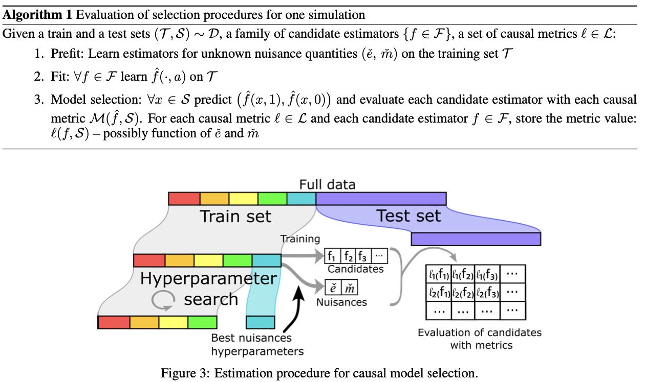
A good causal model-selection procedure: using the so-called R-risk; using flexible estimators to compute the nuisance models on the train set; and splitting out 10% of the data to compute risks.
Note however that they restrict the class of meta-learners (no R-learner for instance) as they claim they compare causal metrics and not optimal learners…
Here is a very nice summary of the estimation procedure:
What can we do from here? Well if there isn’t a clear winner, we might as well look as the most interpretable and actionable metrics, and this is where uplift metrics come into play.
Classic Uplift Metrics
Settings. Let’s start by consider the case of binary treatment \(T\). We try to estimate the cumulative gain of treatment if we were to follow a given policy, possibly trained on historical data.
For a given uplift policy \(\mu\), we ranked unit by decreasing predicted ITE. We denote by \(Y_{i}\) the outcome of unit \(i\) , \(D_i\) (resp. \(D_i^{Treated}\) and \(D_i^{Control}\)) the number of units with predicted ITE less or equal than unit \(i\) (resp. in the treated and control group). For a ranked unit \(k\),
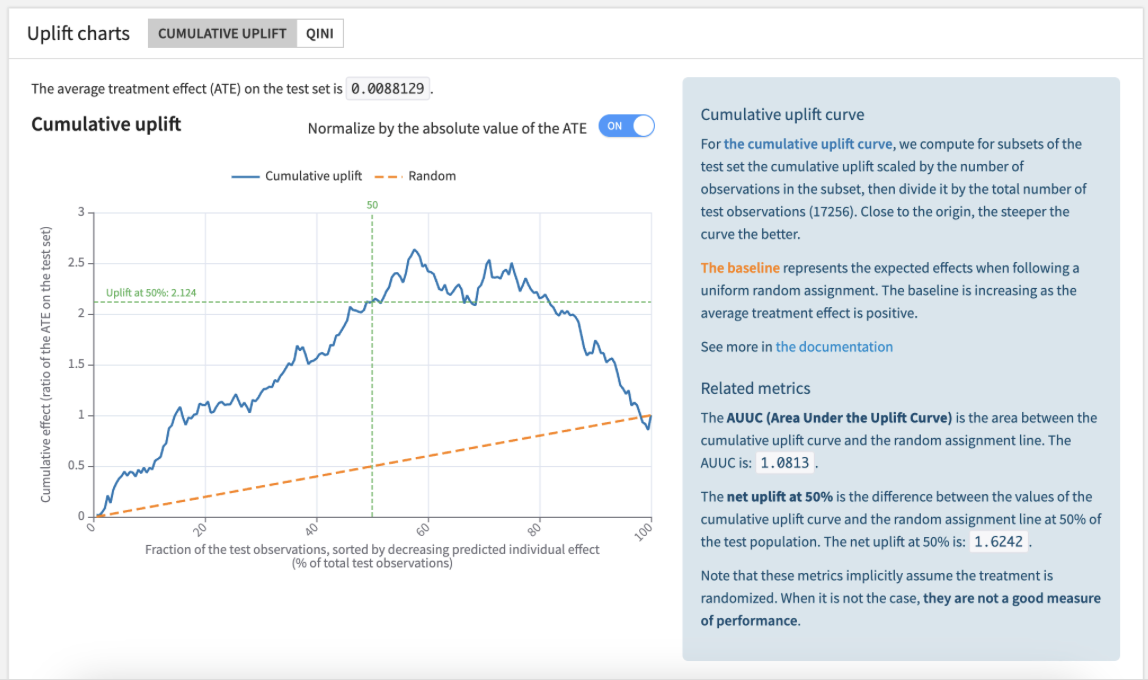
\[Uplift@k := (\frac{\sum_{i=1}^{k}Y_i*\unicode{x1D7D9}_{i \in Treated}}{D_k^{Treated}} - \frac{\sum_{i=1}^{k}Y_i*\unicode{x1D7D9}_{i \in Control}}{D_k^{Control}}) \cdot D_k\]The function \(k \mapsto Uplift@k\) is the so-called uplift curve. Here is what it looks like in Dataiku’s platform.
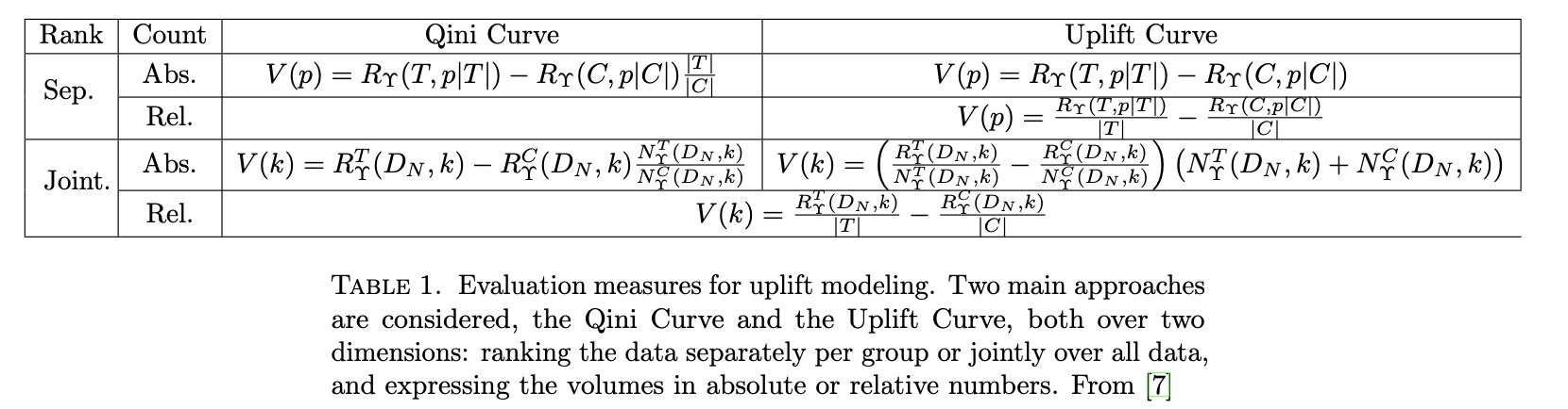
For a complete and rigorous presentation of those metrics and all their variants, this work from Criteo, About Evaluation Metrics for Contextual Uplift modeling is the most comprehensive resource. Those variants are consequence of the choice of normalization and whether the population ranking is done separately over groups or jointly. This is summarized in this table presented in the above paper:
In Learning to Rank For Uplift Modeling, the discrepancies in the literature around Qini/uplift curves is also nicely presented.
We will now discuss three specific points with those metrics: the extension from binary to multi-treatment, the perfect uplift curve and a robust extension to uplift curve.
Extension to Multi-treatment
We now move to multiple treatments settings with still a control. We can extend the previous metric naturally by replacing the left term \(D_i^{Treated}\) with \(D_i^{T=\mu(X)}\), the subpopulation of units that received the treatment that the policy \(\mu\) would have proposed.
\[Uplift@k :=(\frac{\sum_{i=1}^{k}Y_i*\unicode{x1D7D9}_{i \in Treated}}{D_k^{T=\mu(X)}} - \frac{\sum_{i=1}^{k}Y_i*\unicode{x1D7D9}_{i \in Control}}{D_k^{Control}}) \cdot D_k\]For randomized experiment data, this gives an unbiased estimation of the uplift metric (see Lemma 2.1 in Uplift Modeling with Multiple Treatments and General Response Types). Note that this imposes a filtering that might drastically reduces validation dataset size.
In this Uber’s paper Uplift Modeling for Multiple Treatments with Cost Optimization, we see that the binary-treatment policies on the left-hand plot are ending at the same point while the right-hand plot for multi-treatment policies ends at different points.
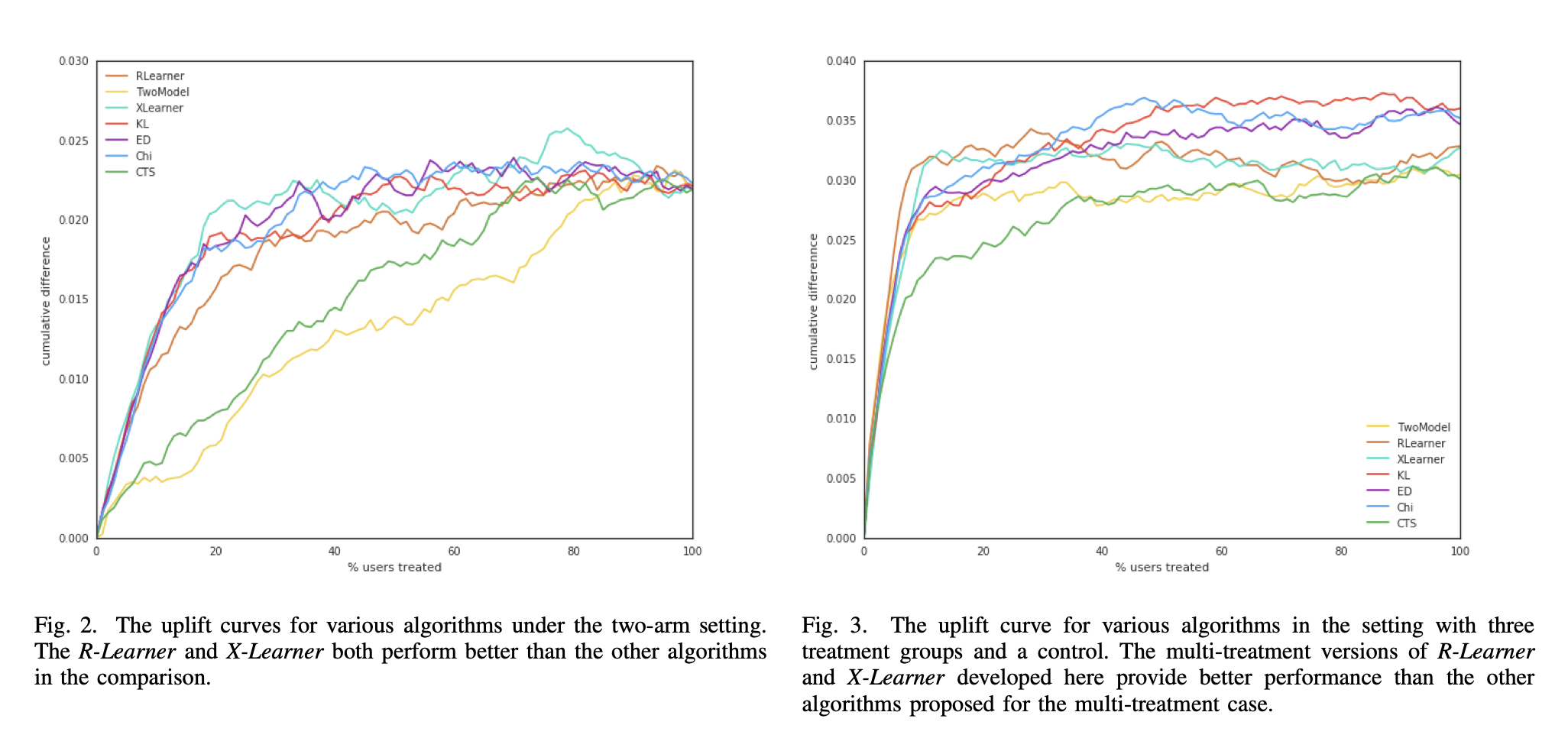
What’s going on ? In binary settings, all uplift metrics end at the global ATE on the validation data, which is not the case for multi-treatment. This means that we need to be very careful in how normalization is done in order to do model selection.
We cannot normalise by the policy’s predicted ATE (the curve’s last point) anymore as this depends on the population policy, which is the control group together with \(D^{T=\mu(X)}\). This normalization makes model comparison impossible4 and we need to control for the total population policy size.
Extensions.
- When doing cross-validation, a better strategy is to do that normalization over each fold and average the folds by the global fold ATE.
- Outside of randomized experiments, but within the bound of unconfoundedness, the above can be generalized with IPW-weighting5.
Note. After writing this, I came across mr_uplift which is a library dedicated to multi-treatment uplift that offer similar metrics.
What’s the perfect uplift curve?
Let’s go back to binary treatment. One of the benefits of uplift curves is that you can define a theoretical perfect policy on the historical data. Of course, this is only a restrospective and not a prescriptive policy but it’s always interesting to have upper bound.
In scikit-uplift, a heuristic perfect uplift curve is proposed. It ranks the four populations (treated/not treated and converted/not converted) and the policy is constant over each population.
Naturally, it first ranks the treated converted and then the control not-converted. We then need to decide who to rank next. We denote the number of control who responded by \(CR\) and the treated who didn’t responded by \(TN\). If \(CR < TN\), it starts with treated not-converted, otherwise it starts with not-converted.
This is under the implicit hypothesis that there are as many treated as control. Indeed, as you can see from this beautiful screenshot, we should control for that ratio (treated/control).

Robust Uplift
In (again) the very nice About Evaluation Metrics for Contextual Uplift modeling, the authors discusses how to deal with segments of the population with same predicted (iso-predicted) uplift.
As suggested we can do linear interpolation for such segments (see python code below) which is a sort of average optimum. Similarly, we could consider the minimum and maxium uplift curve segment which convey a natural uncertainty over those segments.
Another natural extension is to have a looser definition of iso-predicted, and define either a tolerance parameter or a binning.
def constant_segments(x):
    '''Returns locations and segments lengths of constants subsegments in x'''
    x = np.sort(x)

    mask = np.concatenate(([True], x[1:] != x[:-1],[True]))
    nonzero_ix = np.where(mask)[0]

    locations = nonzero_ix[:-1]
    segments_length = np.diff(nonzero_ix)

    return locations, segments_length

def linear_interpolation_smoothing(y, locations, segments_length):
    """Returns a copy of y where constants segments are linearly interpolated"""
    new_y = np.copy(y)
    new_y = new_y.astype(float)

    for i, ix_length in enumerate(segments_length):
        if ix_length>1:
            ix_start = locations[i]

            if ix_start ==0:
                start_value = new_y[ix_start]
                end_value = new_y[ix_start+ix_length-1]
            else:
                start_value = new_y[ix_start-1]
                end_value = new_y[ix_start+ix_length-1]

            slope = (end_value - start_value)/ix_length
            intercept = start_value

            if ix_start ==0:
                linear = slope * np.arange(0,ix_length) + intercept
                new_y[ix_start: ix_start+ix_length] = linear
            else:
                linear = slope * np.arange(1,ix_length) + intercept
                new_y[ix_start: ix_start+ix_length-1] = linear
    return new_y
Last but not least, note that the issues discussed here with metrics for uplift modelling have natural strong connections with offline policy evaluation in Reinforcement Learning, but we’ll leave this for another time…
-
There are others like scikit-uplift, causallift, the now-archived Wayfair librarypylift, or the highly scalable Booking UpliftML. ↩
-
Papers like Mining for the truly responsive customers and prospects using true-lift modeling: Comparison of new and existing methods or From predictive uplift modeling to prescriptive uplift analytics: A practical approach to treatment optimization while accounting for estimation risk… that can be easily found on sci-hub thankfully. ↩
-
We introduced one of the author of the paper (Brady Neal) to Qini scores which was added to a second version of the paper :). ↩
-
Unfortunately this is how normalization is done in causalML at this point. ↩
-
Also presented in the Criteo paper. ↩